rejected posts

You are no longer bound to traditional clinical trials: 21st Century Cures!

.

I was just sent this in my email. Knowing nothing about it, and unable to comment, it’s here in my Rejected Posts alternative blog. I’m keen to hear what others, familiar with it, think of this 21st Century Cures Act. (It reminds me of the Doors, 20th Century Fox). Actually, I think this was passed in 2016, so it’s not big news. Of course the push for “personalized medicine is part of this, never mind that it hasn’t had much success yet. I would have thought observational studies were at least admissible before. Do they require adjustments for data-dredging? Or not? I’m glad they will mention “pitfalls”. Now I’m going to have to ask my doctor which type of study a drug has had its approval based upon.

Thanks to the 21st Century Cures Act you are no longer bound to traditional clinical trials to prove safety and efficacy — new and exciting alternatives are available to you!

Observational studies are now acceptable in the FDA’s approval process.  These studies allow the collection of real-world usage information from patients and physicians. And they allow for the harvesting of data from existing studies — from university research to patient data registries — to use as evidence of a product’s efficacy and safety (my emphasis).

Observational research requires an entirely different set of procedures and careful planning to ensure the real-world evidence collected is valid and reliable.

The 21st Century Take on Observational Studies walks you through everything you need to know about the opportunities and pitfalls observational studies can offer. The report looks at the growing trend toward observational research and how provisions in the 21st Century Cures Act create even more incentives to rely on real-world evidence in the development of medical products. The report covers:

  • Provisions of the 21st Century Cures Act related to observational studies and gathering of real-world evidence
  • The evolution of patient-focused research
  • How observational studies can be used in the preapproval and postmarket stages
  • The potential for saving time and money
  • New data sources that make observational studies a viable alternative to clinical trials
  • How drug- and devicemakers view observational research and how they are using it

Order your copy of The 21st Century Take on Observational Studies: Using Real-World Evidence in the New Millennium and learn effective uses of observational studies in both the preapproval and postmarket phases; how to identify stakeholders and determine what kind of data they needed, and how the FDA’s view on observational research is evolving.

Order your copy today button

Categories: rejected posts | 2 Comments

Souvenirs from “the improbability of statistically significant results being produced by chance alone”-under construction

images-11

.

I extracted some illuminating gems from the recent discussion on my”Error Statistics Philosophy” blogpost, but I don’t have time to write them up, and won’t for a bit, so I’m parking a list of comments wherein the golden extracts lie here; it may be hard to extricate them from over 120 comments later on. (They’re all my comments, but as influenced by readers.) If you do happen wander into my Rejected Posts blog again, you can expect various unannounced tinkering on this post, and the results may not be altogether grammatical or error free. Don’t say I didn’t warn you.


I’m looking to explain how a frequentist error statistician (and lots of scientists) understand

Pr(Test T produces d(X)>d(x); Ho) ≤ p.

You say ” the probability that the data were produced by random chance alone” is tantamount to assigning a posterior probability to Ho, based on a prior) and I say it is intended to refer to an ordinary error probability. The reason it matters isn’t because 2(b) is an ideal way to phrase the type 1 error prob or the attained significance level. I admit it isn’t ideal But the supposition that it’s a posterior leaves one in the very difficult position of defending murky distinctions, as you’ll see in my next thumb’s up and down comment.

You see, for an error statistician, the probability of a test result is virtually always construed in terms of the HYPOTHETICAL frequency with which such results WOULD occur, computed UNDER the assumption of one or another hypothesized claim about the data generation. These are 3 key words.
Any result is viewed as of a general type, if it is to have any non-trivial probability for a frequentist.
Aside from the importance of the words HYPOTHETICAL and WOULD is the word UNDER.

Computing {d(X) > d(x)} UNDER a hypothesis, here, Ho, is not a conditional probability.** This may not matter very much, but I do think it makes it difficult for some to grasp the correct meaning of the intended error probability.

OK, well try your hand at my next little quiz.

…..
**See double misunderstandings about p-valueshttps://normaldeviate.wordpress.com/2013/03/14/double-misunderstandings-about-p-values/

———————————————-


Thumbs up or down? Assume the p-value of relevance is 1 in 3 million or 1 in 3.5 million. (Hint: there are 2 previous comments of mine in this post of relevance.)

  1. only one experiment in three million would see an apparent signal this strong in a universe [where Ho is adequate].
  2. the likelihood that their signal was a result of a chance fluctuation was less than one chance in 3.5 million
  3. The probability of the background alone fluctuating up by this amount or more is about one in three million.
  4. there is only a 1 in 3.5 million chance the signal isn’t real.
  5. the likelihood that their signal would result by a chance fluctuation was less than one chance in 3.5 million
  6. one in 3.5 million is the likelihood of finding a false positive—a fluke produced by random statistical fluctuation
  7. there’s about a one-in-3.5 million chance that the signal they see would appear if there were [Ho adequate].
  8. it is 99.99997 per cent likely to be genuine rather than a fluke.

They use likelihood when they should mean probability, but we let that go.

The answers will reflect the views of the highly respected PVPs–P-value police.

—————————————————


THUMBS UP OR DOWN ACCORDING TO THE P-VALUE POLICE (PVP)

1. only one experiment in three million would see an apparent signal this strong in a universe [where Ho is adequately describes the process].
up

  1. the likelihood that their signal was a result of a chance fluctuation was less than one chance in 3.5 million
    down
  2. The probability of the background alone fluctuating up by this amount or more is about one in three million.
    up
  3. there is only a 1 in 3.5 million chance the signal isn’t real.
    down
  4. the likelihood that their signal would result by a chance fluctuation was less than one chance in 3.5 million
    up
  5. one in 3.5 million is the likelihood of finding a false positive—a fluke produced by random statistical fluctuation
    down (or at least “not so good”)
  6. there’s about a one-in-3.5 million chance that the signal they see would appear if there were no genuine effect [Ho adequate].
    up
  7. it is 99.99997 per cent likely to be genuine rather than a fluke.
    down

I find #3 as a thumbs up especially interesting.

The real lesson, as I see it, is that even the thumbs up statements are not quite complete in themselves, in the sense that they need to go hand in hand with the INFERENCES I listed in an earlier comment, and repeat below. These incomplete statements are error probability statements, and they serve to justify or qualify the inferences which are not probability assignments.

In each case, there’s an implicit principle (severity) which leads to inferences which can be couched in various ways such as:

Thus, the results (i.e.,the ability to generate d(X) > d(x)) indicate(s):

  1. the observed signals are not merely “apparent” but are genuine.
  2. the observed excess of events are not due to background
  3. “their signal” wasn’t (due to) a chance fluctuation.
  4. “the signal they see” wasn’t the result of a process as described by Ho.

If you’re a probabilist (as I use that term), and assume that statistical inference must take the form of a posterior probability*, then unless you’re meticulous about the “was/would” distinction you may fall into the erroneous complement that Richard Morey aptly describes. So I agree with what he says about the concerns. But the error statistical inferences are 1,3,5,7 along with the corresponding error statistical qualification.

For this issue, please put aside the special considerations involved in the Higgs case. Also put to one side, for this exercise at least, the approximations of the models. If we’re trying to make sense out of the actual work statistical tools can perform, and the actual reasoning that’s operative and why, we are already allowing the rough and ready nature of scientific inference. It wouldn’t be interesting to block understanding of what may be learned from rough and ready tools by noting their approximative nature–as important as that is.

*I also include likelihoodists under “probabilists”.

****************************************************

Richard and everyone: The thumb’s up/downs weren’t mine!!! The are Spiegelhalter’s!
http://understandinguncertainty.org/explaining-5-sigma-higgs-how-well-did-they-do

I am not saying I agree with them! I wouldn’t rule #6 thumbs down, but he does. This was an exercise in deconstructing his and similar appraisals, (which are behind principle #2) in order to bring out the problem that may be found with 2(b). I can live with all of them except #8.

Please see what I say about “murky distinctions” in the comment from earlier:
http://errorstatistics.com/2016/03/12/a-small-p-value-indicates-its-improbable-that-the-results-are-due-to-chance-alone-fallacious-or-not-more-on-the-asa-p-value-doc/#comment-139716

****************************************

PVP’s explanation of official ruling on #6

****************************************

The insights to take away from this thumb’s up:
3. The probability of the background alone fluctuating up by this amount or more is about one in three million.

Given that the PVP are touchy about assigning probabilities to “the explanation” it is noteworthy that this is doing just that. Isn’t it?*
Abstract away as much as possible from the particularities of the Higg’s case, which involves a “background,” in order to get at the issue.

3′ The probability that chance variability alone (or the perhaps the random assignment of treatments) produces a difference as or larger than this is about one in 3 million. (The numbers don’t matter.)

In the case where p is very small, the “or larger” doesn’t really add any probability. The “or larger” is needed for BLOCKING inferences to real effects by producing p-values that are not small. But we can keep it in.

3” The probability that chance alone produces a difference as larger or larger than observed is 1 in 3 million (or other very small value).

3”’The probability that a difference this large or larger is produced by chance alone is 1 in 3 million (or other very small value).

I see no difference between 3, 3′, 3” and p”’. (The PVP seem forced into murky distinctions.)

For a frequentist who follows Fisher in avoiding isolated significant results, the “results” = the ability to produce such statistically significant results.

*Qualification: It’s never what the PVP called “explanation” alone, nor the data alone,at least for a sampling theorist-error statistician. It’s the overall test procedure,or even better: my ability to reliably bring about results that are very improbable under Ho”. I render it easy to bring about results that would be very difficult under Ho.

See also my comment below:

http://errorstatistics.com/2016/03/12/a-small-p-value-indicates-its-improbable-that-the-results-are-due-to-chance-alone-fallacious-or-not-more-on-the-asa-p-value-doc/comment-page-1/#comment-139772

The mistake is in thinking we start with the probabilistic question Richard states. I say we don’t. I don’t.

*********************************************

Here it is:


Richard: I want to come back to your first comment:

You wrote:
if I ask “What is the probability that the symptoms are due to heart disease?” I’m asking a straightforward question about whether the probability that the symptoms are caused by an actual case of heart disease, not the probability that I would see the symptoms assuming I had heart disease.

My reply: Stop right after the first comma, before “not the probability.” The real question of interest is: are these symptoms caused by heart disease (not the probability they are).

In setting out to answer the question suppose you found that it’s quite common to have even worse symptoms due to indigestion and no heart disease. This indicates it’s readily explainable without invoking heart disease. That is, in setting out to answer a non-probabilistic question* you frame it as of a general type, and start asking how often would this kind of thing be expected under various scenarios. You appeal to probabilistic considerations to answer your non-probabilistic question, and when you amass enough info, you answer it. Non-probabilistically.

Abstract from the specifics of the example on heart disease which brings in many other considerations.

*You know the answers are open to error, but that doesn’t make the actual question probabilistic.

*********************************

Mar 20, 2016: Look at #1:

  1. only one experiment in three million would see an apparent signal this strong in a universe [where Ho is adequate/true].
    a. This is a big thumb’s up for the PVP. Now I do have one beef with this, and that’s the fact it doesn’t say that the apparent signal is produced by, or because of, or due to, whatever mechanism is described by Ho. This is important, because unless this production connection is there, it’s not an actual p-value. (I’m thinking of that Kadane chestnut on my regular blog where some “result” (say a tsunami) is very improbable,  and it’s alleged one can put any “null” hypothesis Ho at all to the right of “;” (e.g., no Higgs particle), and get a low p-value for Ho.
    The p-value has to be computable because of Ho, that is, Ho assigns the probability to the results.

    b. Now consider: “an apparent signal this strong in a universe where Ho is the case”. The blue words are what the particle physicist means by a “fluke” of that strength. So we get a thumb’s up to:
    only one experiment in three million would see a fluke this strong (i.e., under Ho)
    or
    the probability of seeing a 5 sigma fluke is one in three million.

Laurie: I get you’re drift, and now I see that it arose because of some very central confusions between how different authors of comments on the ASA doc construed the model. I don’t want to relegate that to a mere problem of nomenclature or convention, but nevertheless, I’d like to take it up another time and return to my vacuous claim.

The Pr(P < p; Ho) = p (very small). Or

(1): Pr(Test T yields d(X) > d(x); Ho) = p (very small) This may be warranted by simulation or analytically, so not mere mathematics, and it’s always approximate, but I’m prepared to grant this.

Or, to allude to Fisher:

The probability of bringing about such statistically significant results “at will”, were Ho the case, is extremely small.

Now for the empirical and non-vacuous part (which we are to spoze is shown):

Spoze

(2): I do reliably bring about stat sig results d(X) &gt; d(x). I’ve shown the capability of bringing about results each of which would occur in, say, 1 in 3 million experiments UNDER the supposition that Ho.

(It’s not even the infrequency that matters, but the use of distinct instruments with different assumptions, where errors in one are known to ramify in the at least one other)

I make the inductive inference (which again, can be put in various terms, but pick any one you like):

(3): There’s evidence of a genuine effect.

The move from (1) and (2) to inferring (3) is based on

(4): Claim (3) has passed a stringent or severe test by dint of (1) and (2). In informal cases, the strongest ones, actually, this is also called a strong argument from coincidence.

(4) is full of content and not at all vacuous, as is (2). I admit it’s “philosophical” but also justifiable on empirical grounds. But I won’t get into those now.

These aren’t all in chronological, but rather (somewhat) logical order. What’s the upshot? I’ll come back to this. Feel free to comment.

Categories: danger, rejected posts | 2 Comments

Can today’s nasal spray influence yesterday’s sex practices? Non-replication isn’t nearly critical enough: Rejected post

images-10

Blame it on the nasal spray

Sit down with students or friends and ask them what’s wrong with this study–or just ask yourself–and it will likely leap out. Now I’ve only read the paper quickly, and know nothing of oxytocin (OT) research. That’s why this is in the “Rejected Posts” blog. Plus, I’m writing this really quickly.

You see, I noticed a tweet about how non-statistically significant results are often stored in filedrawers, rarely published, and right away was prepared to applaud the authors for writing on their negative result. Now that I see the nature of the study, and the absence of any critique of the experiment itself (let alone the statistics), I am less impressed. What amazes me about so many studies is not that they fail to replicate but that the glaring flaws in the study aren’t considered! But I’m prepared to be corrected by those who do serious oxytocin research.

In a nutshell: Treateds get OT nasal spray, controls get a placebo spray; you’re told they’re looking for effects on sexual practices, when actually they’re looking for effects on trust bestowed upon experimenters with your answers).

The instructions were the follows: “You will now perform a task on the computer. The instruction concerning this task will appear on screen but if you have any question, do not hesitate. At the end of the computer test, you will have to fill a questionnaire that is in the envelope on your desk. As we want to examine if oxytocin has an influence on sexual practices and fantasies, do not be surprised by the intimate or awkward nature of the questions. Please answer as honestly as possible. You will not be judged. Also do not be afraid of being sincere in your answers, I will not look at your questionnaire, I swear it. It will be handled by one of the guy in charge of the optical reading device who will not be able to identify you (thanks to the coding system). At the end of the experiment, I will bring him all the questionnaires. I will just ask you to put the questionnaire back in the envelope once it is completed. You may close the envelope at the end and, if you want, you may even add tape. There is a tape dispenser on your desk”. There is some examples of questions they were asked to answer: “What was your wildest sex experiment ?”, “Are you satisfied with your sex life? Could you describe it? (frequency, quality,…)” Please report on a 7-point Likert scale (1 = not at all, it disgusts me à 7 = very much, I really like) your willingness to be involved in the following sexual practices: using sex toys, doing a threesome, having sex in public, watch other people having sex, watch porn before or during a sexual intercourse,…”

Imagine you’re a subject in the study. Is there a reason to care if the researcher knows details of your sex life? The presumption is that you do care. But anyone who really cared wouldn’t reveal whatever they deemed so embarrassing. But wait, there’s another crucial element to this experiment.

We’re told: “we want to examine if oxytocin has an influence on sexual practices and fantasies“. You’ve been sprayed with either OT or placebo, and I assume you don’t know which. Suppose OT does influence willingness to engage in wild sex experiments. Being sprayed today couldn’t very well change your previous behavior. So unless they had asked you last week (without spray) and now once again with spray, they can’t be looking for changes on actual practice. But OT spray could make you more willing to say you’re more willing to engage in “the following sexual practices: using sex toys, doing a threesome, having sex in public,…etc. etc.”  It could also influence feelings right now, i.e., how satisfied you feel now that you’ve been “treated”. So since the subject reasons this must be the effect they have in mind, only scores on the “willingness” and “current feelings” questions could be picking up on the OT effect. But high numbers on willingness and feelings questions don’t reflect actual behaviors–unless the OT effect extends to exaggerating about past behaviors, that is, lying about them, in which case, once again, your own actual choices and behaviors in life are not revealed by the questionnaire. Given the tendency of subjects to answer as they suppose the researcher wants, I can imagine higher numbers on such questions (than if they weren’t told they’re examining if OT has an influence on sexual practices). But since the numbers don’t, indeed, can’t reflect true effects on sexual behavior, there’s scarce reason to regard them as private information revealed only to experimenters you trust.  I’ll bet almost no one uses the tape*.

There are many, alternative criticisms of this study. For example, realizing they can’t be studying the influence of sex practices, you already mistrust the experimenter. Share yours.

Let me be clear: I don’t say OT isn’t related to love and trust––it’s active in childbirth, nursing, and, well…whatever. It is, after all, called the ‘love hormone’. My kvetch is with the capability of this study to discern the intended effect.

I say we need to publish analyses showing what’s wrong with the assumption that a given experiment is capable of distinguishing the “effects” of the “treatment” of interest. And what about those Likert scales! These aren’t exactly genuine measurements merely because they’re quantitative.

*It would be funny to look for a correlation between racy answers and tape.

Categories: junk science, rejected posts | 5 Comments

On what “evidence-Based Bayesians” like Gelman really mean: rejected post

images-3

.

How to interpret subjective Bayesians who want to be hard-nosed Bayesians is often like swimming round and round in a funnel of currents where there’s nothing to hold on to. Well, I think I’ve recently stopped the flow and pegged it. Christian Hennig and I have often discussed this (on my regular blog) and something Gelman posted today, linked me to an earlier exchange between he and Christian.

Christian: I came across an exchange between you and Andrew because it was linked to by Andrew on a current blog post 

It really brings out the confusion I have had, we both have had, and which I am writing about right now (in my book), as to what people like Gelman mean when they talk about posterior probabilities. First:

a posterior of .9 to

H: “θ  is positive”

is identified with giving 9 to 1 odds on H.

Gelman had said: “it seems absurd to assign a 90% belief to the conclusion. I am not prepared to offer 9 to 1 odds on the basis of a pattern someone happened to see that could plausibly have occurred by chance”

Then Christian says, this would be to suggest “I don’t believe it” means “it doesn’t agree with my subjective probability” and Christian doubts Andrew could mean that. But I say he does mean that. His posterior probability is his subjective (however evidence-based) probability. ‘

Next the question is, what’s the probability assigned to? I think it is assigned to H:θ > 0

As for the meaning of “this event would occur 90% of the time in the long run under repeated trials” I’m guessing that “this event” is also H. The repeated “trials” allude to a repeated θ generating mechanism, or over different systems each with a θ. The outputs would be claims of form H (or not-H or different assertions about the  θ for the case at hand ), and he’s saying 90% of the time the outputs would be H, or H would be the case. The outputs are not ordinary test results, but states of affairs, namely θ > 0.

Bottom line: It seems to me that all Bayesians all who assign posteriors to parameters (aside from empirical Bayesians) really mean the kind of odds statement that you and I and most people associate with partial -belief or subjective probability. “Epistemic probability” would do as well, but equivocal. It doesn’t matter how terrifically objectively warranted that subjective probability assignment is, we’re talking meaning. And when one finally realizes this is what they meant all along, everything they say is less baffling. What do you think?

——————————————–

Background

Andrew Gelman:

First off, a claimed 90% probability that θ>0 seems too strong. Given that the p-value (adjusted for multiple comparisons) was only 0.2—that is, a result that strong would occur a full 20% of the time just by chance alone, even with no true difference—it seems absurd to assign a 90% belief to the conclusion. I am not prepared to offer 9 to 1 odds on the basis of a pattern someone happened to see that could plausibly have occurred by chance,

Christian Hennig says:

May 1, 2015 at 1:06 pm

“Then the data under discussion (with a two-sided p-value of 0.2), combined with a uniform prior on θ, yields a 90% posterior probability that θ is positive. Do I believe this? No.”

What exactly would it mean to “believe” this? Are you referring to a “true unknown” posterior probability with which you compare the computed one? How would the “true” one be defined?

Later there’s this:
“I am not prepared to offer 9 to 1 odds on the basis of a pattern someone happened to see that could plausibly have occurred by chance, …”
…which kind of suggests that “I don’t believe it” means “it doesn’t agree with my subjective probability” – but knowing you a bit I’m pretty sure that’s not what you meant before. But what is it then?

Categories: Bayesian meanings, rejected posts | 12 Comments

Fraudulent until proved innocent: Is this really the new “Bayesian Forensics”? (ii) (rejected post)

Objectivity 1: Will the Real Junk Science Please Stand Up?

.

I saw some tweets last night alluding to a technique for Bayesian forensics, the basis for which published papers are to be retracted: So far as I can tell, your paper is guilty of being fraudulent so long as the/a prior Bayesian belief in its fraudulence is higher than in its innocence. Klaassen (2015):

“An important principle in criminal court cases is ‘in dubio pro reo’, which means that in case of doubt the accused is favored. In science one might argue that the leading principle should be ‘in dubio pro scientia’, which should mean that in case of doubt a publication should be withdrawn. Within the framework of this paper this would imply that if the posterior odds in favor of hypothesis HF of fabrication equal at least 1, then the conclusion should be that HF is true.”june 2015 update J Forster
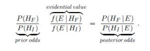
Now the definition of “evidential value” (supposedly, the likelihood ratio of fraud to innocent), called V, must be at least 1. So it follows that any paper for which the prior for fraudulence exceeds that of innocence, “should be rejected and disqualified scientifically. Keeping this in mind one wonders what a reasonable choice of the prior odds would be.”(Klaassen 2015)

Yes, one really does wonder!

“V ≥ 1. Consequently, within this framework there does not exist exculpatory evidence. This is reasonable since bad science cannot be compensated by very good science. It should be very good anyway.”

What? I thought the point of the computation was to determine if there is evidence for bad science. So unless it is a good measure of evidence for bad science, this remark makes no sense. Yet even the best case can be regarded as bad science simply because the prior odds in favor of fraud exceed 1. And there’s no guarantee this prior odds ratio is a reflection of the evidence, especially since if it had to be evidence-based, there would be no reason for it at all. (They admit the computation cannot distinguish between QRPs and fraud, by the way.) Since this post is not yet in shape for my regular blog, but I wanted to write down something, it’s here in my “rejected posts” site for now.

Added June 9: I realize this is being applied to the problematic case of Jens Forster, but the method should stand or fall on its own. I thought rather strong grounds for concluding manipulation were already given in the Forster case. (See Forster on my regular blog). Since that analysis could (presumably) distinguish fraud from QRPs, it was more informative than the best this method can do. Thus, the question arises as to why this additional and much shakier method is introduced. (By the way, Forster admitted to QRPs, as normally defined.) Perhaps it’s in order to call for a retraction of other papers that did not admit of the earlier, Fisherian criticisms. It may be little more than formally dressing up the suspicion we’d have in any papers by an author who has retracted one(?) in a similar area. The danger is that it will live a life of its own as a tool to be used more generally. Further, just because someone can treat a statistic “frequentistly” doesn’t place the analysis within any sanctioned frequentist or error statistical home. Including the priors, and even the non-exhaustive, (apparently) data-dependent hypotheses, takes it out of frequentist hypotheses testing. Additionally, this is being used as a decision making tool to “announce untrustworthiness” or “call for retractions”, not merely analyze warranted evidence.

Klaassen, C. A. J. (2015). Evidential value in ANOVA-regression results in scientific integrity studies. arXiv:1405.4540v2 [stat.ME]. Discussion of the Klaassen method on pubpeer review: https://pubpeer.com/publications/5439C6BFF5744F6F47A2E0E9456703

Categories: danger, junk science, rejected posts | Tags: | 40 Comments

Gelman’s error statistical critique of data-dependent selections–they vitiate P-values: an extended comment

The nice thing about having a “rejected posts” blog, which I rarely utilize, is that it enables me to park something too long for a comment, but not polished enough to be “accepted” for the main blog. The thing is, I don’t have time to do more now, but would like to share my meanderings after yesterday’s exchange of comments with Gelman.

I entirely agree with Gelman that in studies with wide latitude for data-dependent choices in analyzing the data, we cannot say the study was stringently probing for the relevant error (erroneous interpretation) or giving its inferred hypothesis a hard time.

One should specify what the relevant error is. If it’s merely inferring some genuine statistical discrepancy from a null, that would differ from inferring a causal claim. Weakest of all would be merely reporting an observed association. I will assume the nulls are like those in the examples in the “The Garden of Forking Paths” paper, only I was using his (2013) version. I think they are all mere reports of observed associations except for the BEM ESP study. (That they make causal, or predictive, claims already discredits them).

They fall into the soothsayer’s trick of, in effect, issuing such vague predictions that they are guaranteed not to fail.

Here’s a link to Gelman and Loken’s “The Garden of Forking Paths” http://www.stat.columbia.edu/~gelman/research/unpublished/p_hacking.pdf

I agree entirely: “Once we recognize that analysis is contingent on data, the p-value argument disappears–one can no longer argue that, if nothing were going on, that something as extreme as what was observed would occur less than 5% of the time.” (Gelman 2013, p. 10). The nominal p-values does not reflect the improbability of such an extreme or more extreme result due to random noise or “nothing going on”.

A legitimate p-value of α must be such that

Pr(Test yields P-value < α; Ho: chance) ~ α.

With data dependent hypotheses, the probability the test outputs a small significance level can easily be HIGH, when it’s supposed to be LOW. See this post: “Capitalizing on Chance” reporting on Morrison and Henkel from the 1960s!![i]http://errorstatistics.com/2014/03/03/capitalizing-on-chance-2/

Notice, statistical facts about p-values demonstrate the invalidity of taking these nominal p-values as actual. So statistical facts about p-values are self-correcting or error correcting.

So, just as in my first impression of the “Garden” paper, Gelman’s concern is error statistical: it involves appealing to data that didn’t occur, but might have occurred, in order to evaluate inferences from the data that did occur. There is an appeal to a type of sampling distribution over researcher “degrees of freedom” akin to literal multiple testing, cherry-picking, barn-hunting and so on.

One of Gelman’s suggestions is (or appears to be) to report the nominal p-value, and then consider the prior that would render the p-value = to the resulting posterior. If the prior doesn’t seem believable, I take it you are to replace it with one that does. Then, using whatever prior you have selected, report the posterior probability that the effect is real. (In a later version of the paper, there is only reference to using a “pessimistic prior”.) This is remindful of Greenland’s “dualistic” view. Please search on error statistics.com.

Here are some problems I see with this:

  1. The supposition is that for the p-value to be indicative of evidence for the alternative (say in a one-sided test of a 0 null), the p-value should be like a posterior probability for the null, (1- p) to the non-null. This is questionable. http://errorstatistics.com/2014/07/14/the-p-values-overstate-the-evidence-against-the-null-fallacy/

Aside: Why even allow using the nominal p-value as a kind of likelihood to go into the Bayesian analysis if its illegitimate? Can we assume the probability model used to compute the likelihood from the nominal p-value?

  1. One may select the prior in such a way that one reports a low posterior that the effect is real. There’s wide latitude in the selection and it will depend on the framing of the “not-Ho” (non-null).Now one has “critics degrees of freedom” akin to researchers degrees of freedom.

One is not criticizing the study or pinpointing its flawed data dependencies, yet one is claiming to have grounds to criticize it.

Or suppose the effect inferred is entirely believable and now the original result is blessed—even though it should be criticized as having poorly tested the effect. Adjudicating between different assessments by different scientists will become a matter of defending one’s prior, when it should be a matter of identifying the methodological flaws in the study. The researcher will point to many other “replications” in a big field studying similar effects, etc.

There’s a crucial distinction between a poorly tested claim and an implausible claim. An adequate account of statistical testing needs to distinguish these.

I want to be able to say that the effect is quite plausible given all I know, etc., but this was a terrible test of it, and supplies poor grounds for the reality of the effect.

Gelman’s other suggestion, that these experimenters distinguish exploratory from confirmatory experiments, and that they be required to replicate their results is, on the face of it, more plausible. But the only way this would be convincing, as I see it, is if the data analysts were appropriately blinded. Else, they’ll do the same thing with the replication.

I agree of course that a mere nominal p-value “should not be taken literally” (in the sense that it’s not an actual p-value)—but I deny that this is equal to assigning p as a posterior probability to the null.

There are many other cases in which data-dependent hypotheses are well-tested by the same data used in their construction/selection  Distinguishing cases has been the major goal of much of my general work in philosophy of science (and it carries over into PhilStat).

http://errorstatistics.files.wordpress.com/2013/12/mayo-surprising-facts-article-printed-online.pdf

http://errorstatistics.com/2013/12/15/surprising-facts-about-surprising-facts/

 One last thing: Gelman is concerned that the p-values based on these data-dependent associations are misleading the journals and misrepresenting the results. This may be so in the “experimental” cases. But if the entire field knows that this is a data-dependent search for associations that seem indicative of supporting one or another conjecture, and that the p-value is merely a nominal or computed measure of fit, then it’s not clear there is misinterpretation. It’s just a reported pattern.

[i] When the hypotheses are tested on the same data that suggested them and when tests of significance are based on such data, then a spurious impression of validity may result. The computed level of significance may have almost no relation to the true level. . . . Suppose that twenty sets of differences have been examined, that one difference seems large enough to test and that this difference turns out to be “significant at the 5 percent level.” Does this mean that differences as large as the one tested would occur by chance only 5 percent of the time when the true difference is zero? The answer is no, because the difference tested has been selected from the twenty differences that were examined. The actual level of significance is not 5 percent, but 64 percent! (Selvin 1970, 104)


Categories: rejected posts | Tags: | 3 Comments

A SANTA LIVED AS A DEVIL AT NASA! Create an easy peasy Palindrome for December, win terrific books for free!

imagesTo avoid boredom, win a free book, and fulfill my birthday request, please ponder coming up with a palindrome for December. If created by anyone younger than 18, they get to select two books. All it needs to have is one word: math (aside from Elba, but we all know able/Elba). Now here’s a tip: consider words with “ight”: fight, light, sight, might. Then just add some words around as needed. (See rules, they cannot be identical to mine.)

Night am…. math gin

fit sight am ….math gist if

sat fight am…math gift as

You can search “palindrome” on my regular blog for past winners, and some on this blog too.

Thanx, Mayo

Categories: palindrome, rejected posts | 6 Comments

More ironies from the replicationistas: Bet on whether you/they will replicate a statistically significant result

For a group of researchers concerned wit how the reward structure can bias results of significance tests, this has to be a joke or massively ironic:

Second Prediction Market Project for the Reproducibility of Psychological Science

The second prediction market project for the reproducibility project will soon be up and running – please participate!

There will be around 25 prediction markets, each representing a particular study that is currently being replicated. Each study (and thus market) can be summarized by a key hypothesis that is being tested, which you will get to bet on.

In each market that you participate, you will bet on a binary outcome: whether the effect in the replication study is in the same direction as the original study, and is statistically significant with a p-value smaller than 0.05.

Everybody is eligible to participate in the prediction markets: it is open to all members of the Open Science Collaboration discussion group – you do not need to be part of a replication for the Reproducibility Project. However, you cannot bet on your own replications.

Each study/market will have a prospectus with all available information so that you can make informed decisions.

The prediction markets are subsidized. All participants will get about $50 on their prediction account to trade with. How much money you make depends on how you bet on different hypotheses (on average participants will earn about $50 on a Mastercard (or the equivalent) gift card that can be used anywhere Mastercard is used).

The prediction markets will open on October 21, 2014 and close on November 4.

If you are willing to participate in the prediction markets, please send an email to Siri Isaksson by October 19 and we will set up an account for you. Before we open up the prediction markets, we will send you a short survey.

The prediction markets are run in collaboration with Consensus Point.

If you have any questions, please do not hesitate to email Siri Isaksson.

Categories: rejected posts | 3 Comments

Winner of the January 2014 Palindrome Contest

images-5Winner of the January 2014 Palindrome Context

Karthik Durvasula
Visiting Assistant Professor in Phonology & Phonetics at Michigan State University

Palindrome: Test’s optimal? Agreed! Able to honor? O no! hot Elba deer gala. MIT-post set.

The requirement was: A palindrome with “optimal” and “Elba”.

BioI’m a Visiting Assistant Professor in Phonology & Phonetics at Michigan State University. My work primarily deals with probing people’s subconscious knowledge of (abstract) sound patterns. Recently, I have been working on auditory illusions that stem from the bias that such subconscious knowledge introduces.

Statement: “Trying to get a palindrome that was at least partially meaningful was fun and challenging. Plus I get an awesome book for my efforts. What more could a guy ask for! I also want to thank Mayo for being excellent about email correspondence, and answering my (sometimes silly) questions tirelessly.”

Book choice: EGEK 1996! 🙂
[i.e.,Mayo (1996): “Error and the Growth of Experimental Knowledge”]

CONGRATULATIONS! And thanks so much for your interest!

February contest: Elba plus deviate (deviation)

Categories: palindrome, rejected posts | 1 Comment

Sir Harold Jeffreys (tail area) howler: Sat night comedy (rejected post Jan 11, 2014)

IMG_0600You might not have thought there could be yet new material for 2014, but there is: for the first time Sir Harold Jeffreys himself is making an appearance, and his joke, I admit, is funny. So, since it’s Saturday night, let’s listen in on Sir Harold’s howler in criticizing p-values. However, even comics try out “new material” with a dry run, say at a neighborhood “open mike night”. So I’m placing it here under rejected posts, knowing maybe 2 or at most 3 people will drop by. I will return with a spiffed up version at my regular gig next Saturday.

Harold Jeffreys: Using p-values implies that “An hypothesis that may be true is rejected because it has failed to predict observable results that have not occurred.” (1939, 316)

I say it’s funny, so to see why I’ll strive to give it a generous interpretation.

We can view p-values in terms of rejecting H0, as in the joke, as follows:There’s a test statistic D such that H0 is rejected if the observed D,i.e., d0 ,reaches or exceeds a cut-off d* where Pr(D > d*; H0) is very small, say .025. Equivalently, in terms of the p-value:
Reject H0 if Pr(D > d0H0) < .025.
The report might be “reject Hat level .025″.

Suppose we’d reject H0: The mean light deflection effect is 0, if we observe a 1.96 standard deviation difference (in one-sided Normal testing), reaching a p-value of .025. Were the observation been further into the rejection region, say 3 or 4 standard deviations, it too would have resulted in rejecting the null, and with an even smaller p-value. H0 “has not predicted” a 2, 3, 4, 5 etc. standard deviation difference. Why? Because differences that large are “far from” or improbable under the null. But wait a minute. What if we’ve only observed a 1 standard deviation difference (p-value = .16)? It is unfair to count it against the null that 1.96, 2, 3, 4 etc. standard deviation differences would have diverged seriously from the null, when we’ve only observed the 1 standard deviation difference. Yet the p-value tells you to compute Pr(D > 1; H0), which includes these more extreme outcomes. This is “a remarkable procedure” indeed! [i]

So much for making out the howler. The only problem is that significance tests do not do this, that is, they do not reject with, say, D = 1 because larger D values, further from might have occurred (but did not). D = 1 does not reach the cut-off, and does not lead to rejecting H0. Moreover, looking at the tail area makes it harder, not easier, to reject the null (although this isn’t the only function of the tail area): since it requires not merely that Pr(D = d0 ; H0 ) be small, but that Pr(D > d0 ; H0 ) be small. And this is well justified because when this probability is not small, you should not regard it as evidence of discrepancy from the null. Before getting to this, a few comments:

1.The joke talks about outcomes the null does not predict–just what we wouldn’t know without an assumed test statistic, but the tail area consideration arises in Fisherian tests in order to determine what outcomes H0 “has not predicted”. That is, it arises to identify a sensible test statistic D (I’ll return to N-P tests in a moment).

In familiar scientific tests, we know the outcomes that are further away from a given hypothesis in the direction of interest, e.g., the more patients show side effects after taking drug Z, the less indicative it is benign, not the other way around. But that’s to assume the equivalent of a test statistic. In Fisher’s set-up, one needs to identify a suitable measure of closeness, fit, or directional departure. Any particular outcome can be very improbable in some respect. Improbability of outcomes (under H0) should not indicate discrepancy from H0 if even less probable outcomes would occur under discrepancies from H0. (Note: To avoid confusion, I always use “discrepancy” to refer to the parameter values used in describing the underlying data generation; values of D are “differences”.)

2. N-P tests and tail areas: Now N-P tests do not consider “tail areas” explicitly, but they fall out of the desiderata of good tests and sensible test statistics. N-P tests were developed to provide the tests that Fisher used with a rationale by making explicit alternatives of interest—even if just in terms of directions of departure.

In order to determine the appropriate test and compare alternative tests “Neyman and I introduced the notions of the class of admissible hypotheses and the power function of a test. The class of admissible alternatives is formally related to the direction of deviations—changes in mean, changes in variability, departure from linear regression, existence of interactions, or what you will.” (Pearson 1955, 207)

Under N-P test criteria, tests should rarely reject a null erroneously, and as discrepancies from the null increase, the probability of signaling discordance from the null should increase. In addition to ensuring Pr(D < d*; H0) is high, one wants Pr(D > d*; H’: μ0 + γ) to increase as γ increases.  Any sensible distance measure D must track discrepancies from H0.  If you’re going to reason, the larger the D value, the worse the fit with H0, then observed differences must occur because of the falsity of H0 (in this connection consider Kadane’s howler).

3. But Fisher, strictly speaking, has only the null distribution, and an implicit interest in tests with sensitivity of a given type. To find out if H0 has or has not predicted observed results, we need a sensible distance measure.

Suppose I take an observed difference d0 as grounds to reject Hon account of its being improbable under H0, when in fact larger differences (larger D values) are more probable under H0. Then, as Fisher rightly notes, the improbability of the observed difference was a poor indication of underlying discrepancy. This fallacy would be revealed by looking at the tail area; whereas it is readily committed, Fisher notes, with accounts that only look at the improbability of the observed outcome d0 under H0.

4. Even if you have a sensible distance measure D (tracking the discrepancy relevant for the inference), and observe D = d, the improbability of d under H0 should not be indicative of a genuine discrepancy, if it’s rather easy to bring about differences even greater than observed, under H0. Equivalently, we want a high probability of inferring H0 when H0 is true. In my terms, considering Pr(D < d*; H0) is what’s needed to block rejecting the null and inferring H’ when you haven’t rejected it with severity. In order to say that we have “sincerely tried”, to use Popper’s expression, to reject H’ when it is false and H0 is correct, we need Pr(D < d*; H0) to be high.

5. Concluding remarks:

The rationale for the tail area is twofold: to get the right direction of departure, but also to ensure Pr(test T does not reject null; H0 ) is high.

If we don’t have a sensible distance measure D, then we don’t know which outcomes we should regard as those H0 does or does not predict. That’s why we look at the tail area associated with D. Neyman and Pearson make alternatives explicit in order to arrive at relevant test statistics. If we have a sensible D, then Jeffreys’ criticism is equally puzzling because considering the tail area does not make it easier to reject H0 but harder. Harder because it’s not enough that the outcome be improbable under the null, outcomes even greater must be improbable under the null. And it makes it a lot harder (leading to blocking a rejection) just when it should: because the data could readily be produced by H0 [ii].

Either way, Jeffreys’ criticism, funny as it is, collapses.

When an observation does lead to rejecting the null, it is because of that outcome—not because of any unobserved outcomes. Considering other possible outcomes that could have arisen is essential for determining (and controlling) the capabilities of the given testing method. In fact, understanding the properties of our testing tool just is to understand what it would do under different outcomes, under different conjectures about what’s producing the data.


[i] Jeffreys’ next sentence, remarkably is: “On the face of it, the evidence might more reasonably be taken as evidence for the hypothesis, not against it.” This further supports my reading, as if we’d reject a fair coin null because it would not predict 100% heads, even though we only observed 51% heads. But the allegation has no relation to significance tests of the Fisherian or N-P varieties.

[ii] One may argue it should be even harder, but that is tantamount to arguing the purported error probabilities are close to the actual ones. Anyway, this is a distinct issue.

Categories: rejected posts, Uncategorized | 1 Comment

Blog at WordPress.com.