danger

Souvenirs from “the improbability of statistically significant results being produced by chance alone”-under construction

images-11

.

I extracted some illuminating gems from the recent discussion on my”Error Statistics Philosophy” blogpost, but I don’t have time to write them up, and won’t for a bit, so I’m parking a list of comments wherein the golden extracts lie here; it may be hard to extricate them from over 120 comments later on. (They’re all my comments, but as influenced by readers.) If you do happen wander into my Rejected Posts blog again, you can expect various unannounced tinkering on this post, and the results may not be altogether grammatical or error free. Don’t say I didn’t warn you.


I’m looking to explain how a frequentist error statistician (and lots of scientists) understand

Pr(Test T produces d(X)>d(x); Ho) ≤ p.

You say ” the probability that the data were produced by random chance alone” is tantamount to assigning a posterior probability to Ho, based on a prior) and I say it is intended to refer to an ordinary error probability. The reason it matters isn’t because 2(b) is an ideal way to phrase the type 1 error prob or the attained significance level. I admit it isn’t ideal But the supposition that it’s a posterior leaves one in the very difficult position of defending murky distinctions, as you’ll see in my next thumb’s up and down comment.

You see, for an error statistician, the probability of a test result is virtually always construed in terms of the HYPOTHETICAL frequency with which such results WOULD occur, computed UNDER the assumption of one or another hypothesized claim about the data generation. These are 3 key words.
Any result is viewed as of a general type, if it is to have any non-trivial probability for a frequentist.
Aside from the importance of the words HYPOTHETICAL and WOULD is the word UNDER.

Computing {d(X) > d(x)} UNDER a hypothesis, here, Ho, is not a conditional probability.** This may not matter very much, but I do think it makes it difficult for some to grasp the correct meaning of the intended error probability.

OK, well try your hand at my next little quiz.

…..
**See double misunderstandings about p-valueshttps://normaldeviate.wordpress.com/2013/03/14/double-misunderstandings-about-p-values/

———————————————-


Thumbs up or down? Assume the p-value of relevance is 1 in 3 million or 1 in 3.5 million. (Hint: there are 2 previous comments of mine in this post of relevance.)

  1. only one experiment in three million would see an apparent signal this strong in a universe [where Ho is adequate].
  2. the likelihood that their signal was a result of a chance fluctuation was less than one chance in 3.5 million
  3. The probability of the background alone fluctuating up by this amount or more is about one in three million.
  4. there is only a 1 in 3.5 million chance the signal isn’t real.
  5. the likelihood that their signal would result by a chance fluctuation was less than one chance in 3.5 million
  6. one in 3.5 million is the likelihood of finding a false positive—a fluke produced by random statistical fluctuation
  7. there’s about a one-in-3.5 million chance that the signal they see would appear if there were [Ho adequate].
  8. it is 99.99997 per cent likely to be genuine rather than a fluke.

They use likelihood when they should mean probability, but we let that go.

The answers will reflect the views of the highly respected PVPs–P-value police.

—————————————————


THUMBS UP OR DOWN ACCORDING TO THE P-VALUE POLICE (PVP)

1. only one experiment in three million would see an apparent signal this strong in a universe [where Ho is adequately describes the process].
up

  1. the likelihood that their signal was a result of a chance fluctuation was less than one chance in 3.5 million
    down
  2. The probability of the background alone fluctuating up by this amount or more is about one in three million.
    up
  3. there is only a 1 in 3.5 million chance the signal isn’t real.
    down
  4. the likelihood that their signal would result by a chance fluctuation was less than one chance in 3.5 million
    up
  5. one in 3.5 million is the likelihood of finding a false positive—a fluke produced by random statistical fluctuation
    down (or at least “not so good”)
  6. there’s about a one-in-3.5 million chance that the signal they see would appear if there were no genuine effect [Ho adequate].
    up
  7. it is 99.99997 per cent likely to be genuine rather than a fluke.
    down

I find #3 as a thumbs up especially interesting.

The real lesson, as I see it, is that even the thumbs up statements are not quite complete in themselves, in the sense that they need to go hand in hand with the INFERENCES I listed in an earlier comment, and repeat below. These incomplete statements are error probability statements, and they serve to justify or qualify the inferences which are not probability assignments.

In each case, there’s an implicit principle (severity) which leads to inferences which can be couched in various ways such as:

Thus, the results (i.e.,the ability to generate d(X) > d(x)) indicate(s):

  1. the observed signals are not merely “apparent” but are genuine.
  2. the observed excess of events are not due to background
  3. “their signal” wasn’t (due to) a chance fluctuation.
  4. “the signal they see” wasn’t the result of a process as described by Ho.

If you’re a probabilist (as I use that term), and assume that statistical inference must take the form of a posterior probability*, then unless you’re meticulous about the “was/would” distinction you may fall into the erroneous complement that Richard Morey aptly describes. So I agree with what he says about the concerns. But the error statistical inferences are 1,3,5,7 along with the corresponding error statistical qualification.

For this issue, please put aside the special considerations involved in the Higgs case. Also put to one side, for this exercise at least, the approximations of the models. If we’re trying to make sense out of the actual work statistical tools can perform, and the actual reasoning that’s operative and why, we are already allowing the rough and ready nature of scientific inference. It wouldn’t be interesting to block understanding of what may be learned from rough and ready tools by noting their approximative nature–as important as that is.

*I also include likelihoodists under “probabilists”.

****************************************************

Richard and everyone: The thumb’s up/downs weren’t mine!!! The are Spiegelhalter’s!
http://understandinguncertainty.org/explaining-5-sigma-higgs-how-well-did-they-do

I am not saying I agree with them! I wouldn’t rule #6 thumbs down, but he does. This was an exercise in deconstructing his and similar appraisals, (which are behind principle #2) in order to bring out the problem that may be found with 2(b). I can live with all of them except #8.

Please see what I say about “murky distinctions” in the comment from earlier:
http://errorstatistics.com/2016/03/12/a-small-p-value-indicates-its-improbable-that-the-results-are-due-to-chance-alone-fallacious-or-not-more-on-the-asa-p-value-doc/#comment-139716

****************************************

PVP’s explanation of official ruling on #6

****************************************

The insights to take away from this thumb’s up:
3. The probability of the background alone fluctuating up by this amount or more is about one in three million.

Given that the PVP are touchy about assigning probabilities to “the explanation” it is noteworthy that this is doing just that. Isn’t it?*
Abstract away as much as possible from the particularities of the Higg’s case, which involves a “background,” in order to get at the issue.

3′ The probability that chance variability alone (or the perhaps the random assignment of treatments) produces a difference as or larger than this is about one in 3 million. (The numbers don’t matter.)

In the case where p is very small, the “or larger” doesn’t really add any probability. The “or larger” is needed for BLOCKING inferences to real effects by producing p-values that are not small. But we can keep it in.

3” The probability that chance alone produces a difference as larger or larger than observed is 1 in 3 million (or other very small value).

3”’The probability that a difference this large or larger is produced by chance alone is 1 in 3 million (or other very small value).

I see no difference between 3, 3′, 3” and p”’. (The PVP seem forced into murky distinctions.)

For a frequentist who follows Fisher in avoiding isolated significant results, the “results” = the ability to produce such statistically significant results.

*Qualification: It’s never what the PVP called “explanation” alone, nor the data alone,at least for a sampling theorist-error statistician. It’s the overall test procedure,or even better: my ability to reliably bring about results that are very improbable under Ho”. I render it easy to bring about results that would be very difficult under Ho.

See also my comment below:

http://errorstatistics.com/2016/03/12/a-small-p-value-indicates-its-improbable-that-the-results-are-due-to-chance-alone-fallacious-or-not-more-on-the-asa-p-value-doc/comment-page-1/#comment-139772

The mistake is in thinking we start with the probabilistic question Richard states. I say we don’t. I don’t.

*********************************************

Here it is:


Richard: I want to come back to your first comment:

You wrote:
if I ask “What is the probability that the symptoms are due to heart disease?” I’m asking a straightforward question about whether the probability that the symptoms are caused by an actual case of heart disease, not the probability that I would see the symptoms assuming I had heart disease.

My reply: Stop right after the first comma, before “not the probability.” The real question of interest is: are these symptoms caused by heart disease (not the probability they are).

In setting out to answer the question suppose you found that it’s quite common to have even worse symptoms due to indigestion and no heart disease. This indicates it’s readily explainable without invoking heart disease. That is, in setting out to answer a non-probabilistic question* you frame it as of a general type, and start asking how often would this kind of thing be expected under various scenarios. You appeal to probabilistic considerations to answer your non-probabilistic question, and when you amass enough info, you answer it. Non-probabilistically.

Abstract from the specifics of the example on heart disease which brings in many other considerations.

*You know the answers are open to error, but that doesn’t make the actual question probabilistic.

*********************************

Mar 20, 2016: Look at #1:

  1. only one experiment in three million would see an apparent signal this strong in a universe [where Ho is adequate/true].
    a. This is a big thumb’s up for the PVP. Now I do have one beef with this, and that’s the fact it doesn’t say that the apparent signal is produced by, or because of, or due to, whatever mechanism is described by Ho. This is important, because unless this production connection is there, it’s not an actual p-value. (I’m thinking of that Kadane chestnut on my regular blog where some “result” (say a tsunami) is very improbable,  and it’s alleged one can put any “null” hypothesis Ho at all to the right of “;” (e.g., no Higgs particle), and get a low p-value for Ho.
    The p-value has to be computable because of Ho, that is, Ho assigns the probability to the results.

    b. Now consider: “an apparent signal this strong in a universe where Ho is the case”. The blue words are what the particle physicist means by a “fluke” of that strength. So we get a thumb’s up to:
    only one experiment in three million would see a fluke this strong (i.e., under Ho)
    or
    the probability of seeing a 5 sigma fluke is one in three million.

Laurie: I get you’re drift, and now I see that it arose because of some very central confusions between how different authors of comments on the ASA doc construed the model. I don’t want to relegate that to a mere problem of nomenclature or convention, but nevertheless, I’d like to take it up another time and return to my vacuous claim.

The Pr(P < p; Ho) = p (very small). Or

(1): Pr(Test T yields d(X) > d(x); Ho) = p (very small) This may be warranted by simulation or analytically, so not mere mathematics, and it’s always approximate, but I’m prepared to grant this.

Or, to allude to Fisher:

The probability of bringing about such statistically significant results “at will”, were Ho the case, is extremely small.

Now for the empirical and non-vacuous part (which we are to spoze is shown):

Spoze

(2): I do reliably bring about stat sig results d(X) &gt; d(x). I’ve shown the capability of bringing about results each of which would occur in, say, 1 in 3 million experiments UNDER the supposition that Ho.

(It’s not even the infrequency that matters, but the use of distinct instruments with different assumptions, where errors in one are known to ramify in the at least one other)

I make the inductive inference (which again, can be put in various terms, but pick any one you like):

(3): There’s evidence of a genuine effect.

The move from (1) and (2) to inferring (3) is based on

(4): Claim (3) has passed a stringent or severe test by dint of (1) and (2). In informal cases, the strongest ones, actually, this is also called a strong argument from coincidence.

(4) is full of content and not at all vacuous, as is (2). I admit it’s “philosophical” but also justifiable on empirical grounds. But I won’t get into those now.

These aren’t all in chronological, but rather (somewhat) logical order. What’s the upshot? I’ll come back to this. Feel free to comment.

Categories: danger, rejected posts | 2 Comments

Fraudulent until proved innocent: Is this really the new “Bayesian Forensics”? (ii) (rejected post)

Objectivity 1: Will the Real Junk Science Please Stand Up?

.

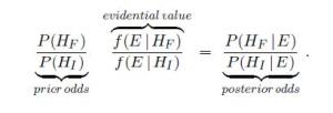
I saw some tweets last night alluding to a technique for Bayesian forensics, the basis for which published papers are to be retracted: So far as I can tell, your paper is guilty of being fraudulent so long as the/a prior Bayesian belief in its fraudulence is higher than in its innocence. Klaassen (2015):

“An important principle in criminal court cases is ‘in dubio pro reo’, which means that in case of doubt the accused is favored. In science one might argue that the leading principle should be ‘in dubio pro scientia’, which should mean that in case of doubt a publication should be withdrawn. Within the framework of this paper this would imply that if the posterior odds in favor of hypothesis HF of fabrication equal at least 1, then the conclusion should be that HF is true.”june 2015 update J ForsterNow the definition of “evidential value” (supposedly, the likelihood ratio of fraud to innocent), called V, must be at least 1. So it follows that any paper for which the prior for fraudulence exceeds that of innocence, “should be rejected and disqualified scientifically. Keeping this in mind one wonders what a reasonable choice of the prior odds would be.”(Klaassen 2015)

Yes, one really does wonder!

“V ≥ 1. Consequently, within this framework there does not exist exculpatory evidence. This is reasonable since bad science cannot be compensated by very good science. It should be very good anyway.”

What? I thought the point of the computation was to determine if there is evidence for bad science. So unless it is a good measure of evidence for bad science, this remark makes no sense. Yet even the best case can be regarded as bad science simply because the prior odds in favor of fraud exceed 1. And there’s no guarantee this prior odds ratio is a reflection of the evidence, especially since if it had to be evidence-based, there would be no reason for it at all. (They admit the computation cannot distinguish between QRPs and fraud, by the way.) Since this post is not yet in shape for my regular blog, but I wanted to write down something, it’s here in my “rejected posts” site for now.

Added June 9: I realize this is being applied to the problematic case of Jens Forster, but the method should stand or fall on its own. I thought rather strong grounds for concluding manipulation were already given in the Forster case. (See Forster on my regular blog). Since that analysis could (presumably) distinguish fraud from QRPs, it was more informative than the best this method can do. Thus, the question arises as to why this additional and much shakier method is introduced. (By the way, Forster admitted to QRPs, as normally defined.) Perhaps it’s in order to call for a retraction of other papers that did not admit of the earlier, Fisherian criticisms. It may be little more than formally dressing up the suspicion we’d have in any papers by an author who has retracted one(?) in a similar area. The danger is that it will live a life of its own as a tool to be used more generally. Further, just because someone can treat a statistic “frequentistly” doesn’t place the analysis within any sanctioned frequentist or error statistical home. Including the priors, and even the non-exhaustive, (apparently) data-dependent hypotheses, takes it out of frequentist hypotheses testing. Additionally, this is being used as a decision making tool to “announce untrustworthiness” or “call for retractions”, not merely analyze warranted evidence.

Klaassen, C. A. J. (2015). Evidential value in ANOVA-regression results in scientific integrity studies. arXiv:1405.4540v2 [stat.ME]. Discussion of the Klaassen method on pubpeer review: https://pubpeer.com/publications/5439C6BFF5744F6F47A2E0E9456703

Categories: danger, junk science, rejected posts | Tags: | 40 Comments

Saturday night comedy from a Bayesian diary (rejected post*)

Breaking through 'the breakthrough'

Breaking through ‘the breakthrough’

A reader sends me this excerpt from Thomas Leonard’s “Bayesian Boy” book or diary or whatever it is:

“While Professor Mayo’s ongoing campaign against LP would appear to be wild and footloose, she has certainly shaken up the Bayesian Establishment.”
 
Maybe the “footloose” part refers to the above image (first posted here.) I actually didn’t think the Bayesian Establishment had taken notice. (My paper on the strong likelihood principle (SLP) is here).
 
*This falls under “rejected posts” since it has no direct PhilStat content. But the links do.
Categories: danger, rejected posts, strong likelihood principle | 10 Comments

A note circulating on the strong likelihood principle (SLP)

Part II: Breaking Through the Breakthrough* (please start with Dec 6 post)(Sneaking this up on “Rejected Posts” when no one’s looking; I took it off my regular blog in July after ….well, e-mail me if you want to know.)

Four different people now have sent me a letter circulating on an ISBA  e-mail list (by statistician Thomas Leonard) presumably because it mentions the (strong) likelihood principle (SLP). Even in exile, those ISBA e-mails reach me, maybe through some Elba-NSA retrieval or simply past connections. I had already written a note to Professor Leonard* about my new paper on the controversial Birnbaum argument.  I’m not sure what to make of the letter (I know nothing about Leonard): I surmise it pertains to a recent interview of Dennis Lindley (of which I watched just the beginning). Anyway, the letter and follow-ups may be found at their website: http://bayesian.org/forums/news/5374.

Dear fellow Bayesians,

Peter Wakker is to be complimented on his deep understanding of
the De Finetti and Lindley-Savage Axiom systems.
Nevertheless

(1) The Likelihood Principle doesn’t need to be justified by any axiom
systems at all. As so elegantly proved by Alan Birnbaum (JASA,1962) , it is
an immediate consequence of the Sufficiency Principle, when applied to a
mixed experiment, and the Conditionality Principle. The frequency arguments
used to prove the Neyman-Fisher factorization theorem substantiiate
this wonderful result

(2) The strong additivity assumptions in the appropriately extended De
Finetti axiom system are, I think, virtually tautologous wih finite
additivity of the prior measure..So why not just assume the latter, and
forget the axioms altogether? The axioms are just window dressing, a
sprinkling of holy water from Avignon, Rome or wherever..

(3) The Sure Thing Principle is an extremely strong assumption, since it
helps to imply the Expected Utility Hypothesis, which has been long since
refuted by the economists. See for example Maurice Allais’ famous 1953
paradox and the other paradoxes described in Ch.4 of my book Bayesian
Methods (with John Hsu, C.U.P.,1999) where one of many reasonable
extensions to the Expected Utility hypthesis is proposed..

When Dennis brought me up to be a Bayesian Boy, he emphasised
the following normative philosophies::

If you want to be coherent you have to be a
(proper) Bayesian

If you’re not a Bayesian, then you’re incoherent.
and a sure loser to boot

Therefore all frequentists are criiminals

(After 1973) So are Bayesiabs who use improper
priors

Sorry, Dennis, but I still don’t believe a word pf it

(Note that the counterexamples to improper priors
described by Stone, Dawid and Zidek, 1973, relate to quite contrived,
anomalous situations,. While some sampling models can only be analysed
using proper priors, a judicious choice of improper prior distribution will
produce a sensible posterior when analysing most standard parametrised
models)

Yours sincerely

Thomas Leonard

Re: Interview with Dennis Lindley

Without wishing to generate any spam, could I possibly add that Michael
Evans (University of Toronto) has advised me that Birnbaum’s 1962
justification of the LP is mathematical unsound, It should be more
correctly stated as

Theorem: If we accept SP and accept CP, and we accept all the equivalences
generated jointly by these principles, then we must accept LP

Michael also proves:

Theorem: If we accept CP and we accept all equivalences generated by CP
then we must accept LP

Therefore all the counterexamples to LP published by Deborah Mayo (Virginia
Tech) are presumably correct. Moreover the extra conditions may be very
difficult to satisfy in practice. History has been made!

Gee whiz, Dennis! Where does that put the mathematical foundations of
Bayesian statistics now? Both De Finetti and Birnbaum have misled us with
their mathematically unsound proofs. I think that either you or Adrian
should break cover and respond to this. And how about the highly misleading
empirical claims in your 1972 paper on M-Group regression which I’ve long
since refuted (e.g. Sun, Hsu, Guttman, and Leonard (1996), and the
inaugural ISBA meeting in San Francisco in 1993)? I call upon you and
Adrian to finally formally retract them in JRSSB..

And now back to my poetry—-

With best wishes to Bayesians and frequentists everywhere,

Thomas Leonard

Writer, Poet, and Statistician

Edinburgh, Scotland


Categories: danger, strong likelihood principle | 3 Comments

APRIL 1, 2013

Explaining my April 1, 2013 blog:

I was alone in my beautiful office at Thebes (where I live)*. I really didn’t have the time to spend on a jokey April 1 post, but given this blog has only been in existence a year and one-half, I felt I should try for some kind of “tradition” on April fool’s day, especially in case I had a great idea next year. Last year 
 http://errorstatistics.com/2012/04/01/3102/ had many fooled, so lest I let people down, I tried to think of a wild joke that related to our topics, and came across “The Sin of Bad Science” –“bad science” being a frequent theme around here.  But the more I read the Tilberg Report to which it led, and passages from Stapel’s book, the less my idea seemed wild after all, but rather, all-too-believable.  I had no time to come up with something else, and decided to design the post with a productive end: to get people to read section 5 of the Report.

The IG is imaginary, but not so far-fetched (given the interviews in the Report). Thus, the April Fool’s joke is partly on me! Finding the European Association letter (a link to which was only added after Kent Staley’s comment on the post) nearly does derail at least part of (what I thought was) my wild and zany idea.

If people do not see how this state of affairs is promoted by the trends in philosophy of science and statistical practice over the last 15 years or so, they should think again. For examples, scan the blog:

For an index to Jan-Feb: http://errorstatistics.com/2013/03/10/blog-contents-2013-jan-feb/.

*Spoof on Diederik’s memoir.

Categories: danger | 1 Comment

Rejected Post: 3 Msc. Kvetches on the Blog Bagel Circuit

mayo-at-deskIn the past week, I’ve kvetched over at 3 of the blogs on my blog bagel (instead of using the time to work). Here are the main ones, you can follow up on their blogs if you wish:

I.  I made a brief comment on a blatant error in Mark Chang’s treatment of my Birnbaum disproof on  Xi’an’s Og. Chang is responding to Christian Robert’s critical review of his book, Paradoxes in Scientific Inference (2013)

Mayo Says: December 27, 2012 at 9:08 am (actually posted Dec.26,~1:30 a.m.)

I have only gotten to look at Mark Chang’s book a few days ago. I have many concerns regarding his treatment of points from Mayo and Spanos (2010), in particular the chapters by Cox and Mayo (2010) and Mayo (2010). Notably, having set out, nearly verbatim (but without quotes), my first variation of Birnbaum’s argument (Mayo 2010, 309), Chang takes, as evidence that “Mayo’s disproof is faulty”, assertions that I make only concerning the second variation of the Birnbaum argument (310-11).  Chang has written (Chang, 138) the first version in detail, but obviously doesn’t understand it. The problem with the first version is that the two premises cannot both be true at the same time (the crucial term shifts its meaning in the two premises). The second formulation, by contrast, allows both premises to be true. I label the two premises of the second variation as (1) and (2)’.  The problem in the second formulation is: “The antecedent of premise (1) is the denial of the antecedent of premise (2)’.”(Mayo 2010, 311). (Note the prime on (2)’. )These are both conditional claims, hence they have antecedents. Chang gives this quote, but has missed its reference. I might mention that I don’t see the relevance of Chang’s point about sufficiency to either variations of Birnbaum’s proof (bottom para, Chang 138).

A less informal and clearer treatment of my Birnbaum argument may be found in a recent paper: On the Birnbaum Argument for the Strong Likelihood Principle. Continue reading

Categories: danger, Misc Kvetching, phil stat | 3 Comments

Are you butter off now?

“Are you butter off now? Deconstructing the butter bust of the President” D. Mayo

I thought the sand sculpture of the President was strange, but this unsalted butter bust of the President being wheeled around Chicago (under the banner of “Harvest”) seems downright creepy.

“If you see a yellow-ish sculpture of a man’s head rolling through the Loop Friday afternoon, your eyes aren’t playing tricks on you: It really is a bust of President Barack Obama made of butter.”

Source: http://www.nbcchicago.com/blogs/ward-room/Butter-Bust-of-Obama-Takes-to-Chicago-Streets-175971941.html#ixzz2AWegVEhW

 “Though one would be right to say that artist Bob Kling is buttering up the President with his high-fat bust of his likeness, the act shouldn’t be considered an endorsement. Continue reading

Categories: danger, rejected posts | Tags: , , | 3 Comments

Blog at WordPress.com.