Notes (from Feb 6*) on the irrelevant conjunction problem for Bayesian epistemologists (i)

images-2


* refers to our seminar: Phil6334

I’m putting these notes under “rejected posts” awaiting feedback and corrections.

Contemporary Bayesian epistemology in philosophy appeals to formal probability to capture informal notions of “confirmation”, “support”, “evidence”, and the like, but it seems to create problems for itself by not being scrupulous about identifying the probability space, set of events, etc. and not distinguishing between events and statistical hypotheses. There is usually a presumed reference to games of chance, but even there things can be altered greatly depending on the partition of events. Still, we try to keep to that. The goal is just to give a sense of that research program. (Previous posts on the tacking paradox: Oct. 25, 2013: “Bayesian Confirmation Philosophy and the Tacking Paradox (iv)*” &  Oct 25.

(0) Simple Bayes Boost R: 

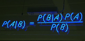
H is “confirmed” or supported by x if P(H|x) > P(H) (P(x |H)) > P(x).

H is disconfirmed (or undermined) by x if P(H|x) < P(H), (else x is confirmationally irrelevant to H).

Mayo: The error statistician would already get off at (0): probabilistic affirming the consequent is maximally unreliable, violating the minimal requirement for evidence. That could be altered with context-depedent information about how the data and hypotheses are arrived at, but this is not made explicit.

(a) Paradox of irrelevant conjunctions (‘tacking paradox’)

If x confirms H, then x also confirms (H & J), even if hypothesis J is just “tacked on” to H.[1]

Hawthorne and Fitelson (2004) define:

J is an irrelevant conjunct to H, with respect to evidence x just in case

P(x|H) = P(x|H & J).

(b) Example from earlier: For instance, x might be radioastronomic data in support of:

H: “the GTR deflection of light effect is 1.75” and

J: “the radioactivity of the Fukushima water dumped in the Pacific ocean is within acceptable levels”.

(1) Bayesian (Confirmation) Conjunction: If x Bayesian confirms H, then x Bayesian-confirms:

(H & J), where P(xH & J ) = P(x|H) for any J consistent with H

(where J is an irrelevant conjunct to H, with respect to evidence x).

If you accept R, (1) goes through.

Mayo: We got off at (0) already.  Frankly I don’t  know why Bayesian epistemologists would allow adding an arbitrary statement or hypothesis not amongst those used in setting out priors. Maybe it’s assumed J is in there somehow (in the background K), but it seems open-ended, and they have not objected.

But let’s just talk about well-defined events in a probability experiment; and limit ourselves to talking about an event providing evidence of another event (e.g., making it more or less expected) in some sense. In one of Fitelson’s examples,   P(black|ace of spade) > P(black), so “black” confirms it’s an ace of spades (presumably in random drawings of card color from an ordinary deck)–despite “ace” being an “irrelevant conjunct” of sorts. Even so, if someone says data x (it’s a stock trader) is evidence it’s an inside trader in a hedge firm, I think it would be assumed that something had been done to probe the added conjuncts.

(2) Using simple B-boost R: (H & J) gets just as much of a boost by x as does H—measuring confirmation as a simple B-boost: R.

CR(H, x) = CR((HJ), x) for irrelevant conjunct J.

R: P(H|x)/P(H) (or equivalently, P(x |H)/P(x))

(a) They accept (1) but (2) is found counterintuitive (by many or most Bayesian epistemologists). But if you’ve defined confirmation as a B-boost, why run away from the implications? (A point Maher makes.) It seems they implicitly slide into thinking of what many of us want:

some kind of an assessment of how warranted or well-tested H is (with x and background).

(not merely a ratio which, even if we can get it, won’t mean anything in particular. It might be any old thing, 2, 22, even with H scarcely making x expected.).

(b) The intuitive objection according to Crupi and Tentori (2010) is this (e.g., p. 3): “In order to claim the same amount of positive support from x to a more committal theory “H and J” as from x to H alone, …adding J should contribute by raising further how strongly x is expected assuming H by itself. Otherwise, what would be the specific relevance of J?” (using my letters, emphasis added)

But the point is that it’s given that J is irrelevant. Now if one reports all the relevant information for the inference, one might report something like (H & J) makes x just as expected as H alone. Why not object to the “too was” confirmation (H & J) is getting when nothing has been done to probe J? I think the objection is, or should be, that nothing has been done to show J is the case rather than not. P(x |(H & J)) = P(x |(H & ~J)).

(c) Switch from R to LR: What Fitelson (Hawthorne and Fitelson 2004) do is employ, as a measure of the B-boost, what some call the likelihood ratio (LR).

CLR(H, x) = P(x | H)/P(x | ~H).

(3) Let x confirm H, then

(*) CLR(H, x) > CLR((HJ), x)

For J an irrelevant conjunct to H.

So even though x confirms (H & J) it doesn’t get as much as H does, at least if one uses LR. (It does get as much using R).

They see (*) as solving the irrelevant conjunct problem.

(4) Now let x disconfirm Q, and x confirm ~Q, then

(*) CLR(~Q, x) > CLR((~Q & J), x)

For J an irrelevant conjunct to Q: P(x|Q) = P(x|J & Q).

Crupi and Tentori (2010) notice an untoward consequence of using LR confirmation in the case of disconfirmation (substituting their Q for H above): If x disconfirms Q, then (Q & J) isn’t as badly disconfirmed as Q is, for J an irrelevant conjunct to Q. But this just follows from (*), doesn’t it? That is, from (*), we’d get (**) [possibly an equality goes somewhere.)

(**) CLR(Q, x) < CLR((Q & J), x).

This says that if x disconfirms Q, (Q & J) isn’t as badly disconfirmed as Q is. This they find counterintuitive.

But if (**) is counterintuitive, then so is (*).

(5) Why (**) makes sense if you wish to use LR:

The numerators in the LR calculations are the same:

P(x|Q & J) = P(x|Q) and P(x|H & J) = P(x|H) since in both cases J is an irrelevant conjunct.

But P(x|~(Q & J)) < P(x|~Q)

Since x disconfirms Q, x is more probable given ~Q than it is given (~Q v ~J). This explains why

(**) CLR(Q, x) < CLR((Q & J), x)

So if (**) is counterintuitive then so is (*).

(a) Example Qunready for college.

If x = high scores on a battery of college readiness tests, then x disconfirms Q and confirms ~Q.

What should J be? Suppose having one’s favorite number be an even number (rather than an odd number) is found irrelevant to scores.

(i) P(x|~(Q & J)) = P(high scores| either college ready or ~J)

(ii) P(x|~Q ) = P(high scores| college ready)

(ii) might be ~1 (as in the earlier discussion), while (i) considerable less.

The high scores can occur even among those whose favorite number is odd.This explains why

(**) CLR(Q, x) < CLR((Q & J), x)

In the case where x confirms H, it’s reversed

P(x |~(H & J)) > P(x |~H)

(b) Using one of Fitelson’s examples, but for ~Q:

e.g., Q: not-spades    x: black      J: ace

P(x |~Q) = 1.

P(x | Q)= 1/3

P(x |~(Q & J)) = 25/49

i.e., P(black|spade or not ace)=25/49

Note: CLR [(Q & J), x) = P(x |(Q & J))/P(x |~(Q & J))

Please share corrections, questions.

Previous slides are:

http://errorstatistics.com/2014/02/09/phil-6334-day-3-feb-6-2014/

http://errorstatistics.com/2014/01/31/phil-6334-day-2-slides/

REFERENCES:

Chalmers (1999). What Is This Thing Called Science, 3rd ed. Indianapolis; Cambridge: Hacking.

Crupi & Tentori (2010). Irrelevant Conjunction: Statement and Solution of a New Paradox, Phil Sci, 77, 1–13.

Hawthorne & Fitelson (2004). Re-Solving Irrelevant Conjunction with Probabilistic Independence, Phil Sci 71: 505–514.

Maher (2004). Bayesianism and Irrelevant Conjunction, Phil Sci 71: 515–520.

Musgrave (2010) “Critical Rationalism, Explanation, and Severe Tests,” in Error and Inference (D.Mayo & A. Spanos eds). CUP: 88-112.


[1] Chalmers and Musgrave say I should make more of how simply severity solves it, notably for distinguishing which pieces of a larger theory rightfully receive evidence, and a variety of “idle wheels” (Musgrave, p. 110.)

Categories: phil6334 rough drafts | 3 Comments

Winner of the January 2014 Palindrome Contest

images-5Winner of the January 2014 Palindrome Context

Karthik Durvasula
Visiting Assistant Professor in Phonology & Phonetics at Michigan State University

Palindrome: Test’s optimal? Agreed! Able to honor? O no! hot Elba deer gala. MIT-post set.

The requirement was: A palindrome with “optimal” and “Elba”.

BioI’m a Visiting Assistant Professor in Phonology & Phonetics at Michigan State University. My work primarily deals with probing people’s subconscious knowledge of (abstract) sound patterns. Recently, I have been working on auditory illusions that stem from the bias that such subconscious knowledge introduces.

Statement: “Trying to get a palindrome that was at least partially meaningful was fun and challenging. Plus I get an awesome book for my efforts. What more could a guy ask for! I also want to thank Mayo for being excellent about email correspondence, and answering my (sometimes silly) questions tirelessly.”

Book choice: EGEK 1996! 🙂
[i.e.,Mayo (1996): “Error and the Growth of Experimental Knowledge”]

CONGRATULATIONS! And thanks so much for your interest!

February contest: Elba plus deviate (deviation)

Categories: palindrome, rejected posts | 1 Comment

Sir Harold Jeffreys (tail area) howler: Sat night comedy (rejected post Jan 11, 2014)

IMG_0600You might not have thought there could be yet new material for 2014, but there is: for the first time Sir Harold Jeffreys himself is making an appearance, and his joke, I admit, is funny. So, since it’s Saturday night, let’s listen in on Sir Harold’s howler in criticizing p-values. However, even comics try out “new material” with a dry run, say at a neighborhood “open mike night”. So I’m placing it here under rejected posts, knowing maybe 2 or at most 3 people will drop by. I will return with a spiffed up version at my regular gig next Saturday.

Harold Jeffreys: Using p-values implies that “An hypothesis that may be true is rejected because it has failed to predict observable results that have not occurred.” (1939, 316)

I say it’s funny, so to see why I’ll strive to give it a generous interpretation.

We can view p-values in terms of rejecting H0, as in the joke, as follows:There’s a test statistic D such that H0 is rejected if the observed D,i.e., d0 ,reaches or exceeds a cut-off d* where Pr(D > d*; H0) is very small, say .025. Equivalently, in terms of the p-value:
Reject H0 if Pr(D > d0H0) < .025.
The report might be “reject Hat level .025″.

Suppose we’d reject H0: The mean light deflection effect is 0, if we observe a 1.96 standard deviation difference (in one-sided Normal testing), reaching a p-value of .025. Were the observation been further into the rejection region, say 3 or 4 standard deviations, it too would have resulted in rejecting the null, and with an even smaller p-value. H0 “has not predicted” a 2, 3, 4, 5 etc. standard deviation difference. Why? Because differences that large are “far from” or improbable under the null. But wait a minute. What if we’ve only observed a 1 standard deviation difference (p-value = .16)? It is unfair to count it against the null that 1.96, 2, 3, 4 etc. standard deviation differences would have diverged seriously from the null, when we’ve only observed the 1 standard deviation difference. Yet the p-value tells you to compute Pr(D > 1; H0), which includes these more extreme outcomes. This is “a remarkable procedure” indeed! [i]

So much for making out the howler. The only problem is that significance tests do not do this, that is, they do not reject with, say, D = 1 because larger D values, further from might have occurred (but did not). D = 1 does not reach the cut-off, and does not lead to rejecting H0. Moreover, looking at the tail area makes it harder, not easier, to reject the null (although this isn’t the only function of the tail area): since it requires not merely that Pr(D = d0 ; H0 ) be small, but that Pr(D > d0 ; H0 ) be small. And this is well justified because when this probability is not small, you should not regard it as evidence of discrepancy from the null. Before getting to this, a few comments:

1.The joke talks about outcomes the null does not predict–just what we wouldn’t know without an assumed test statistic, but the tail area consideration arises in Fisherian tests in order to determine what outcomes H0 “has not predicted”. That is, it arises to identify a sensible test statistic D (I’ll return to N-P tests in a moment).

In familiar scientific tests, we know the outcomes that are further away from a given hypothesis in the direction of interest, e.g., the more patients show side effects after taking drug Z, the less indicative it is benign, not the other way around. But that’s to assume the equivalent of a test statistic. In Fisher’s set-up, one needs to identify a suitable measure of closeness, fit, or directional departure. Any particular outcome can be very improbable in some respect. Improbability of outcomes (under H0) should not indicate discrepancy from H0 if even less probable outcomes would occur under discrepancies from H0. (Note: To avoid confusion, I always use “discrepancy” to refer to the parameter values used in describing the underlying data generation; values of D are “differences”.)

2. N-P tests and tail areas: Now N-P tests do not consider “tail areas” explicitly, but they fall out of the desiderata of good tests and sensible test statistics. N-P tests were developed to provide the tests that Fisher used with a rationale by making explicit alternatives of interest—even if just in terms of directions of departure.

In order to determine the appropriate test and compare alternative tests “Neyman and I introduced the notions of the class of admissible hypotheses and the power function of a test. The class of admissible alternatives is formally related to the direction of deviations—changes in mean, changes in variability, departure from linear regression, existence of interactions, or what you will.” (Pearson 1955, 207)

Under N-P test criteria, tests should rarely reject a null erroneously, and as discrepancies from the null increase, the probability of signaling discordance from the null should increase. In addition to ensuring Pr(D < d*; H0) is high, one wants Pr(D > d*; H’: μ0 + γ) to increase as γ increases.  Any sensible distance measure D must track discrepancies from H0.  If you’re going to reason, the larger the D value, the worse the fit with H0, then observed differences must occur because of the falsity of H0 (in this connection consider Kadane’s howler).

3. But Fisher, strictly speaking, has only the null distribution, and an implicit interest in tests with sensitivity of a given type. To find out if H0 has or has not predicted observed results, we need a sensible distance measure.

Suppose I take an observed difference d0 as grounds to reject Hon account of its being improbable under H0, when in fact larger differences (larger D values) are more probable under H0. Then, as Fisher rightly notes, the improbability of the observed difference was a poor indication of underlying discrepancy. This fallacy would be revealed by looking at the tail area; whereas it is readily committed, Fisher notes, with accounts that only look at the improbability of the observed outcome d0 under H0.

4. Even if you have a sensible distance measure D (tracking the discrepancy relevant for the inference), and observe D = d, the improbability of d under H0 should not be indicative of a genuine discrepancy, if it’s rather easy to bring about differences even greater than observed, under H0. Equivalently, we want a high probability of inferring H0 when H0 is true. In my terms, considering Pr(D < d*; H0) is what’s needed to block rejecting the null and inferring H’ when you haven’t rejected it with severity. In order to say that we have “sincerely tried”, to use Popper’s expression, to reject H’ when it is false and H0 is correct, we need Pr(D < d*; H0) to be high.

5. Concluding remarks:

The rationale for the tail area is twofold: to get the right direction of departure, but also to ensure Pr(test T does not reject null; H0 ) is high.

If we don’t have a sensible distance measure D, then we don’t know which outcomes we should regard as those H0 does or does not predict. That’s why we look at the tail area associated with D. Neyman and Pearson make alternatives explicit in order to arrive at relevant test statistics. If we have a sensible D, then Jeffreys’ criticism is equally puzzling because considering the tail area does not make it easier to reject H0 but harder. Harder because it’s not enough that the outcome be improbable under the null, outcomes even greater must be improbable under the null. And it makes it a lot harder (leading to blocking a rejection) just when it should: because the data could readily be produced by H0 [ii].

Either way, Jeffreys’ criticism, funny as it is, collapses.

When an observation does lead to rejecting the null, it is because of that outcome—not because of any unobserved outcomes. Considering other possible outcomes that could have arisen is essential for determining (and controlling) the capabilities of the given testing method. In fact, understanding the properties of our testing tool just is to understand what it would do under different outcomes, under different conjectures about what’s producing the data.


[i] Jeffreys’ next sentence, remarkably is: “On the face of it, the evidence might more reasonably be taken as evidence for the hypothesis, not against it.” This further supports my reading, as if we’d reject a fair coin null because it would not predict 100% heads, even though we only observed 51% heads. But the allegation has no relation to significance tests of the Fisherian or N-P varieties.

[ii] One may argue it should be even harder, but that is tantamount to arguing the purported error probabilities are close to the actual ones. Anyway, this is a distinct issue.

Categories: rejected posts, Uncategorized | 1 Comment

Winner of the December 2013 palindrome book contest

fxxnmzg-1WINNER: Zachary David
PALINDROME:
Ableton Live: ya procedure plaid, yo. Oy, dial Peru decor. Pay evil, not Elba.

Zachery notes: “Ableton Live is a popular DJ software all the hipster kids use.”

MINIMUM REQUIREMENT**: A palindrome that includes Elba plus procedure.

BIO: Zachary David is a quantitative software developer at a Chicago-based proprietary trading firm and a student at Northwestern University. He infrequently blogs at http://zacharydavid.com.

BOOK SELECTION: “I’d love to get Error and Inference* off of my wish list and onto my desk.”

EDITOR: It’s yours!

STATEMENT: “Finally, after years of living in Wicker Park, my knowledge of hipsters has found its way into poetry and paid out in prizes. I would like to give a special thank you to professor Mayo for being very welcoming to this first time palindromist. I will definitely participate again… I enjoyed the mental work out. Perhaps the competition will pick up in the future.”

*Full title of book choice:

Error and Inference: Recent Exchanges on Experimental Reasoning, Reliability and the Objectivity and Rationality of Science (by D. G. Mayo and A. Spanos, eds.,CUP 2010), 

Note: The word for January 2014 is “optimal” (plus Elba). See January palindrome page.

Congratulations Zachary!

**Nor can it repeat or be close to one that Mayo posts. Joint submissions are permitted (1 book); no age requirements. Professional palindromists not permitted to enter. Note: The rules became much easier starting May 2013, because no one was winning, or even severely trying. The requirements had been Elba + two selected words, rather than only one. I hope we can go back to the more severe requirements once people get astute at palindromes—it will increase your verbal IQ, improve mental muscles, and win you free books. (The book selection changes slightly each month).

_________

Categories: Uncategorized | 1 Comment

Mascots of Bayesneon statistics (rejected post)

bayes_theoremBayes-neon Mascots (desperately seeking): a neon sign! puppies! wigless religious figureprobably the reverend!

I have always thought that the neon sign (of the definition of conditional probability)–first spotted on a truly impressive cult blog–is the fitting emblem for a certain subset of contemporary Bayes: neon. Politically, epistemologically, and commercially–it says it all!

(My “proper” blog (compared to this one) has a stock mascot, Diamond Offshore. Unfortunately, it’s at like a year low. Search rejected posts, if interested in the story. The insignia or pictorial emblem for that blog is the exiled one, casting about for inductive insights):

photo-2-fishing

Categories: rejected posts | 2 Comments

Saturday night comedy from a Bayesian diary (rejected post*)

Breaking through 'the breakthrough'

Breaking through ‘the breakthrough’

A reader sends me this excerpt from Thomas Leonard’s “Bayesian Boy” book or diary or whatever it is:

“While Professor Mayo’s ongoing campaign against LP would appear to be wild and footloose, she has certainly shaken up the Bayesian Establishment.”
 
Maybe the “footloose” part refers to the above image (first posted here.) I actually didn’t think the Bayesian Establishment had taken notice. (My paper on the strong likelihood principle (SLP) is here).
 
*This falls under “rejected posts” since it has no direct PhilStat content. But the links do.
Categories: danger, rejected posts, strong likelihood principle | 10 Comments

PhilStock: No-pain bull

imagesPhilStock. I haven’t had time for stock research in the past 6 months, but fortunately, no changes to portfolios have been required. With Yellen’s assurances last week that the monthly methadone injections of $85 billion[i] of  will continue, it’s bull, bull, bull, with new highs weekly. Even my airlines—generally the worst area to trade in—are, yes flying high (e.g., American from $1.90 to over $11., Delta, Jet Blue, all soaring). But look how low our Diamond Offshore mascot (DO) is [ii]. It is said that small investors typically jump into the market only after the bull has been running:

“The likely outcome is they’ll ride that last-gasp bull market for a short while and experience an enormous loss in personal wealth when the bubble collapses.”(link)

I’m guessing the next 4 months might be safe (T, VZ, WIN?): Remember, though, the one rule on PhilStock: Never ever listen to (i.e., act on) anything I say about the stock market.

[i]in monthly bond market purchases.

[ii] There’s an explanation (of course). It hardly matters with over 5% in special dividends. For why DO is the “mascot” of my regular blog, search rejected posts.

Some related posts:
Bad News is Good News on Wallstreet

Topsy-turvy game

The great taper caper

Categories: phil stock, rejected posts, Uncategorized | Leave a comment

A note circulating on the strong likelihood principle (SLP)

Part II: Breaking Through the Breakthrough* (please start with Dec 6 post)(Sneaking this up on “Rejected Posts” when no one’s looking; I took it off my regular blog in July after ….well, e-mail me if you want to know.)

Four different people now have sent me a letter circulating on an ISBA  e-mail list (by statistician Thomas Leonard) presumably because it mentions the (strong) likelihood principle (SLP). Even in exile, those ISBA e-mails reach me, maybe through some Elba-NSA retrieval or simply past connections. I had already written a note to Professor Leonard* about my new paper on the controversial Birnbaum argument.  I’m not sure what to make of the letter (I know nothing about Leonard): I surmise it pertains to a recent interview of Dennis Lindley (of which I watched just the beginning). Anyway, the letter and follow-ups may be found at their website: http://bayesian.org/forums/news/5374.

Dear fellow Bayesians,

Peter Wakker is to be complimented on his deep understanding of
the De Finetti and Lindley-Savage Axiom systems.
Nevertheless

(1) The Likelihood Principle doesn’t need to be justified by any axiom
systems at all. As so elegantly proved by Alan Birnbaum (JASA,1962) , it is
an immediate consequence of the Sufficiency Principle, when applied to a
mixed experiment, and the Conditionality Principle. The frequency arguments
used to prove the Neyman-Fisher factorization theorem substantiiate
this wonderful result

(2) The strong additivity assumptions in the appropriately extended De
Finetti axiom system are, I think, virtually tautologous wih finite
additivity of the prior measure..So why not just assume the latter, and
forget the axioms altogether? The axioms are just window dressing, a
sprinkling of holy water from Avignon, Rome or wherever..

(3) The Sure Thing Principle is an extremely strong assumption, since it
helps to imply the Expected Utility Hypothesis, which has been long since
refuted by the economists. See for example Maurice Allais’ famous 1953
paradox and the other paradoxes described in Ch.4 of my book Bayesian
Methods (with John Hsu, C.U.P.,1999) where one of many reasonable
extensions to the Expected Utility hypthesis is proposed..

When Dennis brought me up to be a Bayesian Boy, he emphasised
the following normative philosophies::

If you want to be coherent you have to be a
(proper) Bayesian

If you’re not a Bayesian, then you’re incoherent.
and a sure loser to boot

Therefore all frequentists are criiminals

(After 1973) So are Bayesiabs who use improper
priors

Sorry, Dennis, but I still don’t believe a word pf it

(Note that the counterexamples to improper priors
described by Stone, Dawid and Zidek, 1973, relate to quite contrived,
anomalous situations,. While some sampling models can only be analysed
using proper priors, a judicious choice of improper prior distribution will
produce a sensible posterior when analysing most standard parametrised
models)

Yours sincerely

Thomas Leonard

Re: Interview with Dennis Lindley

Without wishing to generate any spam, could I possibly add that Michael
Evans (University of Toronto) has advised me that Birnbaum’s 1962
justification of the LP is mathematical unsound, It should be more
correctly stated as

Theorem: If we accept SP and accept CP, and we accept all the equivalences
generated jointly by these principles, then we must accept LP

Michael also proves:

Theorem: If we accept CP and we accept all equivalences generated by CP
then we must accept LP

Therefore all the counterexamples to LP published by Deborah Mayo (Virginia
Tech) are presumably correct. Moreover the extra conditions may be very
difficult to satisfy in practice. History has been made!

Gee whiz, Dennis! Where does that put the mathematical foundations of
Bayesian statistics now? Both De Finetti and Birnbaum have misled us with
their mathematically unsound proofs. I think that either you or Adrian
should break cover and respond to this. And how about the highly misleading
empirical claims in your 1972 paper on M-Group regression which I’ve long
since refuted (e.g. Sun, Hsu, Guttman, and Leonard (1996), and the
inaugural ISBA meeting in San Francisco in 1993)? I call upon you and
Adrian to finally formally retract them in JRSSB..

And now back to my poetry—-

With best wishes to Bayesians and frequentists everywhere,

Thomas Leonard

Writer, Poet, and Statistician

Edinburgh, Scotland


Categories: danger, strong likelihood principle | 3 Comments

Bad news is good news on Wall St.

Financial Chart and Line Graph

Topsy turvy again! It was widely predicted that today was the day most likely for Bernanke to announce long-awaited plans to begin “tapering” the $85 billion of monthly bond buying stimulus [i]. But, no. Apparently the economy is more worrisome than Ben expected when he all but declared tapering would be announced at the September meeting. Tapering is delayed, forecasts are lowered; stock market climbs to new highs. Things are so bad (in the economy), they’re good (on Wall St.) Does this make sense?*

[i] “See, “The Great Taper-Caper”.

*Of course, I understand all-too-well why this is happening, but it’s still topsy turvy and rather insane…

Categories: phil stock, rejected posts | 10 Comments

The Great Taper Caper

Financial Chart and Line GraphToday, 2 pm: possible clues to the big market mystery revolving around the word “taper”:

“In the last month alone, the words ‘federal reserve’ and some form of the word ‘taper’ appeared in 1,923 news articles in the Nexis database (the number was 12 in the same period last year)” (link is here).

“The taper caper,” as all stock market sleuths know, is the mystery of whether/when Ben Bernanke will taper off the rate of bond buying, down from the current $85 billion a month. (See my last rejected post.) Investors, traders, and especially trading robots who run the market, are on hair trigger alert for clues from Bernanke today. “And the word on everyone’s lips on Wall Street all morning will be ‘taper‘”. With hints Ben will be departing in 2014, the drama is raised a notch, but the band of (mostly) day traders here at this NYC meet-up are playing it cool…. Tune in later.*

*2:30 pm: Big applause erupts here and doubles of Elba Grease all around!**

**3:15pm Oh-oh…things are good enough to start t-a-a-pering soon, but not right away…oh like it’s a big surprise…topsy turvey coming…buy bonds?

3:20: Mayo departs for furniture shopping at the NY Design Center…***

***5pm: Mayo checks market: Oy, (major plummet!) see what I mean (about topsy turvey)? Glad I bought those tapered bookcases (in ebony macasa). At least they offer something concrete!

Now tomorrow, it will be said the robots overreacted…

Categories: phil stock, rejected posts | 2 Comments

Blog at WordPress.com.